CREATE-AAS Science In Brief: Measurements of Transported Wildfire Pollution in Eureka

Author: Tyler Wizenberg, PhD Candidate, University of Toronto

The high Arctic is often viewed as a pristine, untouched wilderness, far away from human influence. However, in reality this is not always the case and large-scale atmospheric circulation patterns can enable both human-emitted and natural pollution to be swept-up and carried far north. One common form of this transported pollution is the smoke plumes generated by large wildfires at southerly latitudes. These smoke plumes typically contain a wide variety of reactive trace-gases which are photochemically and radiatively active, and which can potentially influence the Arctic climate and environment. Because of this, it is important that we identify, monitor and study these wildfire events as they pass over the high Arctic.

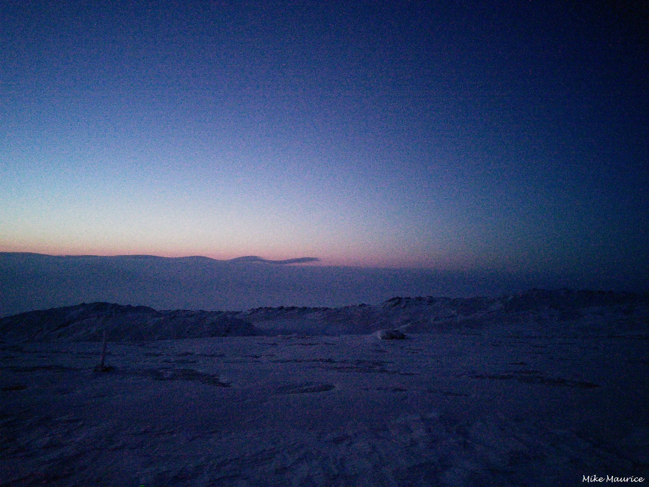
Zeppelin station at Ny-Ålesund on Svalbard, Norway during clear conditions (left), and during hazy conditions caused by transported pollution from agricultural fires in Eastern Europe in May 2006 [1].

How do we measure wildfire pollution?

To measure these wildfire smoke plumes, scientists employ a wide range of tools, the most common of which are: in-situ measurements (i.e. instruments which draw in the surrounding air and chemically analyze the constituents), ground-based remote sensing instruments (i.e. instruments that look upwards and which measure the emitted, absorbed or reflected light passing through the atmosphere), and satellite-borne remote-sensing instruments (similar to the ground-based instruments, but which look downwards towards the Earth or horizontally towards the Earth’s horizon). In the Arctic, we typically rely on the latter two forms of observations since in-situ measurements often must be made close to (and down-wind from) the fire source, and work best when there are many in-situ observation points surrounding the fire.

At the Polar Environment Atmospheric Research Laboratory (PEARL) in Eureka, NU (80.05°N, 86.42°W), we have a Bruker IFS 125HR high-resolution Fourier-transform infrared (FTIR) spectrometer which can measure a broad range of trace-gases that can be detected in the mid and near-infrared wavelengths. This instrument is a powerful tool for identifying wildfire pollution events, and quantifying the magnitude of the pollution relative to normal levels. The Bruker 125HR has been making measurements at PEARL since 2006. This long data record can even allow us to look back and identify past wildfire events which had previously gone unnoticed. Complementing our ground-based measurements are satellites in polar and high-inclination orbits that frequently measure near PEARL, including the Atmospheric Chemistry Experiment (ACE). Accordingly, PEARL is situated at an ideal latitude for validating satellite measurements.

So how do we identify these wildfire pollution events?

In order for us to identify these wildfire smoke plumes in our ground-based FTIR data record, we make use of what can be called “fire tracing species”. An ideal fire tracing species is one which is emitted in large quantities during a forest fire, and which remains in the atmosphere long enough to allow it to be transported up to the high Arctic. Examples of these are carbon monoxide (CO), hydrogen cyanide (HCN) and ethane (C2H6), all of which are typically emitted in significant quantities during a wildfire.

When we observe simultaneous unusually large spikes (or “enhancements”) in these species above their usual levels, it provides strong evidence that we are making measurements within a smoke plume. Over the course of our 2006-2020 data record, we have observed the pollution from multiple fires, including Russian fires in 2008 and 2010, as well as from the Northwest territories fires in 2014. However, these earlier fire events are dwarfed by one that we measured in August 2017. This particular pollution event was the focus of a 2019 publication by one of our team’s former members, Erik Lutsch.

Enhancements of carbon monoxide, ethane, hydrogen cyanide and ammonia (NH3) observed in August 2017 by the PEARL Bruker 125HR. The average yearly trend is given by the black lines [2].

This fire pollution event was actually the result of two individual large-scale wildfires, one in the Northwest territories, and one in British Columbia. In his paper, Erik used a combination of ground-based measurements, satellite observations and chemical transport models to demonstrate that these enhancements can in-fact be traced back to both the B.C. and Northwest territories wildfires.

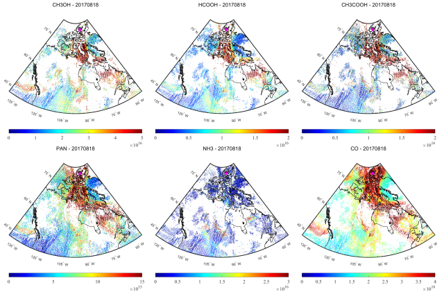
Enhancements in several fire tracing species as seen by the Infrared Atmospheric Sounding Interferometer (IASI) satellite instruments on August 18, 2017 over the Canadian high Arctic. The location of PEARL is marked by a small purple star. Figure courtesy of Bruno Franco, ULibre, Belgium.

In addition to this, through his work Erik established that wildfires can be a substantial source of ammonia to the high Arctic during the summer months. The Arctic has very few natural sources of ammonia (primarily just emissions from the guano of large seabird colonies), so a significant influx of reactive nitrogen in the form of wildfire ammonia pollution can have drastic effects on the sensitive high Arctic ecosystem.

For more details on this exciting new research, feel free to have a look at Erik’s publication on this work.

References

[1] Law, K. S., & Stohl, A. (2007). Arctic Air Pollution: Origins and Impacts. Science, 315(5818), 1537-1540. doi:10.1126/science.1137695

[2] Lutsch, E., Strong, K., Jones, D. B., Ortega, I., Hannigan, J. W., Dammers, E., . . . Fisher, J. A. (2019). Unprecedented Atmospheric Ammonia Concentrations Detected in the High Arctic From the 2017 Canadian Wildfires. Journal of Geophysical Research: Atmospheres, 124(14), 8178-8202. doi:10.1029/2019jd030419

CREATE-AAS Science In Brief: On Improving Measurements of Atmospheric Water Vapour

Author: Dr. Ellen Eckert, Postdoctoral Fellow, University of Toronto

When atmospheric scientists aim to improve measurements of an atmospheric quantity like water vapour, they commonly start off by examining the quality of new observations. This step is called validation. For this, they need a sound understanding of the quantity itself:

How is it distributed throughout the atmosphere? How can it be detected, based on its chemical and physical features, for example using its “spectral fingerprint”? Which chemical reactions is it involved in? How does it influence the atmosphere’s radiation budget? And how do changes in the concentration of an atmospheric gas like water vapour effect Earth’s climate?

In addition to the quantity itself, scientists need to take the impact of different instruments and measurement techniques into account:

Is an instrument measuring directly where it is (in-situ), such as a radiosonde? Or is it measuring water vapour concentrations from a distant location (remote sensing) and thus observing a large volume, like looking at Earth’s atmosphere from a satellite?

Different measurement approaches return different results, even when measuring the same thing. You will probably never get a perfect match even if two different instruments measure the same parcel of air. However, being aware of the differences and the effects they have on the measurements enables scientists to take them into account. Some of these differences can be tackled mathematically, while others are important for interpreting the results of the comparisons.

Why measure water vapour?

Water vapour is highly variable in the atmosphere and plays a significant role in the hydrological cycle. When the Sun heats water in the oceans, lakes and rivers, water vapour evaporates into the atmosphere. It can also evaporate from soil and be transpired from plants. When humid air rises and cools, the water vapour condenses to water droplets, which eventually fall back towards the surface as rain, snow, or other forms of precipitation.

Eureka radiosonde water vapour profiles (January 2007 to December 2017). DJF: December-January-February; MAM: March-April-May; JJA: June-July-August; SON: September-October-November [1]

Besides taking part in atmospheric chemistry and dynamics, water vapour is the most important greenhouse gas in the troposphere and lower stratosphere. Due to climate change, concentrations in stratospheric water vapour are expected to increase, and being able to detect these changes accurately is very important.

But haven’t we been measuring water vapour for quite some time by now?

Yes and no. Even though radiosondes are launched every day from about 1000 stations globally, these ground-based measurements only sample water vapour at specific locations.

Global radiosonde launch sites [from http://www.weather.gov/jetstream/radiosondes ].

The coverage is particularly sparse in remote regions like the Canadian Arctic. In contrast, satellites can provide near-global coverage, but before using these measurements for scientific studies, we have to make sure that they operate to certain standards. This is where ground-based measurements come in handy, because they can be used as a reference for space-borne observation platforms.

One of our team’s former members, Dan Weaver, studied the water vapour measurements made by two instruments on the Atmospheric Chemistry Experiment (ACE) aboard the Canadian atmospheric satellite SCISAT, the Fourier Transform Spectrometer (ACE-FTS) and the Measurement of Aerosol Extinction in the Stratosphere and Troposphere Retrieved by Occultation (MAESTRO). He compared them with radiosonde measurements from the Eureka Weather Station and ground-based remote sensing measurements taken with the Bruker 125HR instrument at the Polar Environment Atmospheric Research Laboratory (PEARL).

Eureka meteorological technicians preparing a weather balloon and a radiosonde for launch. The balloon is filled with hydrogen just before launch and expands as the balloon rises to higher altitudes. The radiosonde takes measurements frequently on its way up and provides detailed information on the vertical distribution of several atmospheric quantities. [Photo: Erik Lutsch]

The Bruker 125HR spectrometer – the T-shaped instrument in the front –  is part of PEARL’s permanent instrument suite. Sunlight is directed down from the roof of the lab to the Bruker 125HR, which uses the physics principle of interference to detect a variety of atmospheric trace gases, including water vapour. [Photo: Erik Lutsch]

Dan was particularly interested in the upper troposphere and lower stratosphere because changes in the concentration of water vapour in this region have a significant impact on how much sunlight, particularly the portion reflected from the Earth’s surface, is absorbed by the atmosphere.

This work discovered that ACE-FTS detects slightly higher amounts of water vapour than the Bruker 125HR in the range of 8-14 km. This is called a ‘wet bias’. For the vertical range of 7-9 km, very good agreement was found between ACE-FTS and the Bruker 125HR. When ACE-FTS was compared with the radiosonde measurements, the results confirmed a ‘wet bias’ above 10 km.

Comparisons with the other instrument on ACE, MAESTRO, turned out to be challenging.

To put these results into perspective, Dan also compared the ACE data with measurements from several other satellites. He was then able to make recommendations on how the data could be used best for scientific applications, for example when looking at a longer time period, and to recommend additional instrumentation that would improve validation studies in the future.

If you would like dig further into the details, feel encouraged to check out Dan’s publication on this research.

References:

 [1] Weaver, D., Strong, K., Schneider, M., Rowe, P. M., Sioris, C., Walker, K. A., Mariani, Z., Uttal, T., McElroy, C. T., Vömel, H., Spassiani, A., and Drummond, J. R.: Intercomparison of atmospheric water vapour measurements at a Canadian High Arctic site, Atmos. Meas. Tech., 10, 2851–2880, https://doi.org/10.5194/amt-10-2851-2017, 2017.

[2] Weaver, D., Strong, K., Walker, K. A., Sioris, C., Schneider, M., McElroy, C. T., Vömel, H., Sommer, M., Weigel, K., Rozanov, A., Burrows, J. P., Read, W. G., Fishbein, E., and Stiller, G.: Comparison of ground-based and satellite measurements of water vapour vertical profiles over Ellesmere Island, Nunavut, Atmos. Meas. Tech., 12, 4039–4063, https://doi.org/10.5194/amt-12-4039-2019, 2019.

The Polar Environment Atmospheric Research Laboratory: PEARL

Author: Dr. Pierre Fogal, PEARL Site Manager, University of Toronto

Stop me if you’ve heard this one before … A bunch of grad students fly into the High Arctic and …

They find everything they need!

So, how does this come to pass?  Well in this case, it is because they are travelling to the Polar Environment Atmospheric Research Laboratory, better known as PEARL!  At PEARL, they walk into a well equipped, moderately comfortable research establishment that supports state-of-the-art laboratory-grade research equipment, as well as the scientists who operate that equipment. PEARL, as you may know, is located at approximately 80.03 degrees North and 86.42 degrees West. It’s a very large distance from the universities that these students attend, and yet there it is, ready for them.  How and why is this the case?  The ‘why’ is fairly straightforward – it is located in a part of the world that is very important to understanding the global atmosphere and is very much under-sampled. The ‘how’ is a more challenging story.

Part of the 2020 ACE/OSIRIS sunrise campaign in front of the Ridge Lab in Eureka, Nunavut. Image Credit: Ramina Alwarda

First of all, PEARL consists of three separate facilities.  The best known of these, the big red building, is sometimes referred to directly as PEARL, although to be precise it is now the PEARL Ridge Laboratory.  The other two facilities are the Zero Altitude PEARL Auxiliary Laboratory (0PAL) and the Surface Atmospheric Flux and IRradiance Extension (SAFIRE).  Back in the beginning when the Canadian Network for Detection of Atmospheric Change (CANDAC) first established PEARL, we thought we would be all about the big red building, but soon after, a need to be near sea-level (the Ridge Lab is at 610 m) was identified, leading to 0PAL, followed then by a need for a site remote from other things with lots of flat space around it and that led to SAFIRE.  0PAL and SAFIRE were constructed by CANDAC based on ISO standard 20-foot long sea-containers, also known as seatainers, while the Ridge Laboratory was constructed in the early 1990s as the Arctic Stratospheric Ozone Observatory (AStrO) by Environment Canada (EC), as it was known then. CANDAC began operating inside AStrO after it was moth-balled by EC.

The Zero Altitude PEARL Auxilary Laboratory (0PAL) in Eureka, Nunavut. Image Credit: Tyler Wizenberg

Given that PEARL is located 400 km north of the most northern settlement in Canada, and about 500 km north of the most northern commercial air terminus, how is it kept operating?  Well, this takes a significant amount of effort on the part of the PEARL operations staff.  The most visible of these are the on-site operators, currently John and Andrew.  They are charged with the day-to-day hands-on verification of instrument operation and status.  They serve as the eyes and ears of the science teams located at the universities and laboratories around Canada and abroad.  They relate what is happening back to the users in the south (just about everywhere is south from PEARL) and then they take action as instructed from the south.  When teams like our aforementioned students arrive, the operators are there to make sure they have what they need and that they can get to where they need to go … and then that they make it back to base in time for meals.

The Surface and Atmospheric Flux, Irradiance and Radiation Extension (SAFIRE) about 5 km from the Eureka Weather Station. Image Credit: Dan Weaver

The planning for deployments happens in the south at headquarters.  There you will find a repository of extreme cold-weather gear, the computer data management systems, specialized instrument support and general expertise that can be drawn upon. Planning for a campaign such as the annual Sunrise satellite validation effort will generally start in mid to late December, and take up a significant part of January.  Any equipment to be shipped north to Yellowknife will generally have to be on its way north by around the last week of January.  Requests for quotations for an aircraft charter from Yellowknife to Eureka will also go out about then.  Flights and hotels for Yellowknife are booked soon after.  The same is done again for the trip home in mid-March.  The same sort of effort is carried out again for summer and fall campaigns.  The summer campaign is the time usually reserved for looking after the facilities and as well as taking the opportunity to do science.  That time of year has 24 hours of daylight, and tends to be A LOT WARMER!

In addition to the science activities, the operations team is also responsible for vehicles to move the team around from weather station to the three sites.  One of the vehicles is specially modified to carry water to the Ridge Laboratory and sewage away from it.  It is not always pleasant, but it is always necessary.  Items too large, or otherwise restricted from flying, travel to Eureka aboard the annual sea-lift. Sea-lift usually occurs in the latter part of August into early September, depending upon scheduling, weather and ice conditions. Sea-lift requires a Canadian Coast Guard ice-breaker, either as the primary vessel or as an escort for a merchant vessel.

The water truck transports water to the Ridge Lab and sewage away from it. Image Credit: Ellen Eckert

It should also be said that the presence of the Environment and Climate Change Canada Eureka Weather Station and personnel greatly simplify the operations at PEARL. Having the support of heavy equipment for snow clearing, road maintenance and building maintenance makes year-round operation feasible.  Additionally, the team will sleep and eat at the Weather Station and the staff are always welcoming of students and CANDAC personnel.

So, those students who walk off that chartered plane walk into a well-organized, controlled environment that is constructed to provide them with the necessities of life.  However, don’t be misled! While it is mostly comfortable, it does require all participants to be careful and vigilante.  Fortunately, all are helpful and all contribute to looking after those around them. Together, those efforts make it possible to work safely and effectively in an otherwise difficult environment!

 

Measuring Arctic Ozone with a Differential Absorption Lidar

Author: Ghazal Farhani, PhD Student at The University of Western Ontario

Ozone is a minor constituent of the atmosphere, but it plays an important role by absorbing harmful ultraviolet (UV) radiation emitted by the Sun. The bulk of this protective ozone resides in the stratosphere at an altitude range between 15 and 50 km. A small amount resides near the surface, but it is a pollutant. Significant chemical depletion of the total ozone during late winter and spring has been observed in both Antarctica and, more recently, in the Arctic. This depletion is commonly known as an ozone hole. The greatest changes in stratospheric ozone occur during polar sunrise (the transition from continuous night to continuous day). In order to detect and quantify the ozone hole, continuous measurements during this period are required.

The ultraviolet beam of the Ozone DIAL at the Ridge Lab in Eureka, Nunavut. Image Credit: Ghazal Farhani

Many different instruments have been used to make ozone measurements. A LiDAR (LIght Detection And Ranging) is one of these instruments. A Lidar is a ground-based active remote sensing instrument that is similar to radar but operates in the ultraviolet, optical, or infrared range. During lidar measurements, laser pulses are sent into the atmosphere, the backscattered photons are collected by a telescope and then detected by photomultiplier tubes. Measurements of the ozone vertical distribution are carried out using a DIfferential Absorption Lidar (DIAL). The high spatial resolution of the receiving signal gives us the opportunity to collect more data to retrieve the ozone profile, and is the big advantage of lidars over satellites.

Observations of stratospheric ozone have been carried out using the DIAL for more than 20 years in Eureka, Nunavut at the Polar Environment Atmospheric Research Laboratory (PEARL). The DIAL system measures ozone by obtaining back-scattered light from two laser wavelengths. One wavelength is in a spectral region with a high absorption for ozone (308 nm), and the other with a low absorption (353 nm). The transmitted laser beam undergoes Rayleigh scattering in the atmosphere and the back-scattered photons are detected by the lidar receiver. Ozone density profiles can be derived from the back-scattered photon measurements.

PhD Student Ghazal Farhani operating the Ozone DIAL. Image Credit: Dr. Emily McCullough

During 2009 and 2010, the laser component of the lidar was replaced and several other components of the lidar were upgraded. As of fall 2014, many of these components have been reinstalled. The refurbished DIAL’s first measurements were made by Dr. Alexey Thikhorimov (Dalhousie University) in February/March 2015 during the ACE/OSIRIS Arctic Validation Campaign.

PhD student Ghazal Farhani checking the Ozone DIAL’s telescope and making sure it’s ready for work.

In the February/March 2016 ACE/OSIRIS Arctic Validation Campaign, Dr. Emily McCullough and I joined Dr. Alexey Thikhomirov to take more measurements. As mentioned above, the DIAL system has been gone through hardware and software replacements. As a result, the data collected from the upgraded system should be validated as well. My PhD thesis will involve learning how to operate the system, and validating the new data. We hope this upgrade will give us better insight into how Ozone concentrations are evolving in the Arctic.

Is there an Arctic ozone hole?

By Kristof Bognar
PhD Candidate, U. of Toronto

When scientists speak of the ‘ozone hole’, they usually mean the large region of low stratospheric ozone concentration that develops above Antarctica each Southern Hemisphere spring (August–October). These occur because conditions over Antarctica are favorable for ozone destruction. Strong westerly winds, or jet streams, above the Southern Ocean circle the continent creating a persistent polar vortex that isolates the air above Antarctica (a twin to the Arctic polar vortex). As this isolated air gets colder and colder, Polar Stratospheric Clouds (PSCs) can form.  PSCs are made up of water ice or nitric acid particles, and reactions occur on the surfaces of these particles that release chlorine compounds from reservoir species.

Polar Stratospheric Clouds (PSCs) above Norway. Since these clouds are at very high altitudes (15000-25000 m), they receive and reflect sunlight from below the horizon. Photo: Ivar Marthinusen, via spaceweathergallery.com.

Chlorine then builds up inside the vortex, and when the Sun rises again in the spring, the molecules are destroyed by photolysis. The released Cl atoms then break down ozone via the reaction cycle pictured below. Since the air above the pole is isolated until the vortex breaks up in late spring, large scale ozone destruction continues as long as it’s cold enough (below -78 °C) for PSCs to exist.

Reactions between chlorine and ozone. A single chlorine atom can destroy thousands of ozone molecules. Source

The atmosphere above the North Pole is much less isolated than the air over Antarctica. The northern polar jet passes over land instead of ocean, and the uneven topography creates a meandering, wavy jet stream pattern and an irregular, variable vortex. The mixing of polar and mid-latitude air prevents the arctic stratosphere from becoming too cold, so PSCs are much less likely to form or persist than in the south. While the underlying chemical processes are the same above both poles, the differences in the evolution of the polar vortex lead to radically different outcomes for stratospheric ozone concentrations.

Daily total ozone concentrations above Antarctica in September 2011 (Southern Hemisphere spring). The blue areas represent ozone depleted air that correlates well with the location of the polar vortex. Note the relatively regular shape and size of these blue areas. Source

Ozone is destroyed above the Arctic every spring, but the net loss is far less than what would be required for an ozone hole.The benchmark total ozone concentration for an ozone hole is 220 Dobson Units (DU). Normal ozone levels are roughly 300 DU globally. Over Antarctica ozone concentrations drop to an average of 100 DU every spring. In the Arctic, however, such dramatic ozone loss is unprecedented, and this is due to the local meteorology.

Daily total ozone concentrations above the Arctic in March 2011 (Northern Hemisphere spring). Once again, the blue areas represent ozone depleted air inside the polar vortex. Note the irregular shapes: the Arctic vortex is more variable than its Antarctic pair. Ozone depletion is also less severe, even though 2011 was a record year in the Arctic. Source.

What’s more, due to transport of warmer, ozone rich air into the vortex in the winter, ozone concentrations in the Arctic are actually the highest in spring. It would require chemical loss comparable to Antarctic levels to bring concentrations even close to an ozone hole. That is, however, exactly what happened in 2010/2011. Due to unusually cold stratospheric conditions, ozone concentrations as low as 220 DU were observed in late March, prompting researchers to acknowledge the existence of the first (and so far only) Arctic ozone hole (Manney et al., 2011).

Monthly average ozone concentrations above both poles. Left: The Arctic in March 2011 (NH spring). Right: Antarctica in September 2011 (SH spring). 2011 saw the most Arctic ozone destruction on record, yet the resulting  ‘ozone hole’ is nowhere near as pronounced as above Antarctica. Source.

This event was also seen by ground based spectrometers at Eureka. These instruments only sample the portion of the vortex directly overhead, but even so they have observed ozone concentrations as low as 237 DU (Adams et al., 2011). 2011 was an exceptional year, since normal springtime ozone concentrations are around 400 DU above the Arctic.

Ozone measurements by two ground-based spectrometers at Eureka. The plots show the number of measurements that returned the given ozone concentrations between Feb. 24 and March 21. The grey columns represent the average values from 1999 to 2010, and the white columns are the 2011 measurements. From Adams et al., 2011.

The variability of the Arctic stratosphere is not well understood, and predicting when the next unusually cold winter might happen is difficult. In February it looked like this spring could bring record ozone losses again (Hand, 2016), but a sudden stratospheric warming in early March and a vortex split mid-March put an end to such speculations. In the future, as the stratosphere cools due to climate change, extremely cold winters might become even colder. So while the Arctic ozone hole has been a one-time phenomenon so far, it has the potential to become a more regular occurrence. Since plenty of people live in the northern parts of the US, Canada, Europe and Russia, strong UV radiation (the consequence of low ozone concentrations) could potentially be harmful if the polar vortex strayed over populated areas. Researchers are working tirelessly to evaluate these risks and predict when and if such events will occur.

References:

Manney, Gloria L., et al. “Unprecedented Arctic ozone loss in 2011.” Nature 478.7370 (2011): 469-475.

Adams, C., et al. “Severe 2011 ozone depletion assessed with 11 years of ozone, NO2, and OClO measurements at 80 N.” Geophysical Research Letters 39.5 (2012).

Hand, Eric. “Record ozone hole may open over Arctic in the spring.” Science 351.6274 (2016): 650-650.

Eureka’s dramatically changing sunlight

By Dan Weaver
Ph.D. Candidate, University of Toronto

You have likely noticed the days are getting longer._­¹ It’s a welcome relief from the short dark days of winter. Toronto, for example, will enjoy over 12 hours of sunlight on April 20. Two months earlier there was only 9.5 hours of sunlight. The seasonal change in sunlight hours is small near the equator, and larger as latitude increases. In the high Arctic, where a Canadian research team is conducting fieldwork at the Polar Environment Atmospheric Research Laboratory (PEARL), the sunlight shift is extreme.

The dramatic transition in sunlight hours between Polar Night and the Midnight Sun in Eureka, Nunavut. Lines note the start and end dates of the 2016 Eureka ACE/OSIRIS Validation Campaign.

The pre-campaign team arrived at PEARL on Saturday, February 20 – the last day of Polar Night. There hadn’t been any sunlight yet in 2016. That quickly changed. A week later, on February 27, the intensive phase research team had their first day at PEARL, having arrived the previous evening. Watching the sunrise and sunset was very convenient that day: sunrise was at 10:15 AM; the sun set at 3:45 PM. That’s five and a half hours of sunlight. On the intensive phase team’s last day at PEARL (March 18) there was over 12 hours of sunlight: the sun rose before 7 AM and set after 7 PM. A couple of team members will stay an additional two weeks. On their last day, April 1, the sun will rise at ~4:30 AM and set ~9:15 PM. There will be nearly 17 hours of sunlight!

Dan Weaver and Joseph Mendonca watch the sun rise on February 25, 2013 (Credit: Paul Loewen)

A variety of PEARL instruments, such as the Cimel sun photometer and the Bruker 125 high resolution (FTIR) spectrometer, use sunlight to measure the atmosphere. As the sunlight hours increase, scientists are able to take more and more data. (Other instruments don’t depend on sunlight, but they have other limitations).

Sunrise (lower data) and sunset times (upper data) during the dramatic transition from Polar Night to Midnight Sun in Eureka, Nunavut (2016).

One of PEARL’s technicians wrote an interesting blog last year about his experience working in complete darkness during Polar Night, and watching as the landscape slowly revealed itself throughout February.

Why does this happen?

Every year, the Earth’s axis tilts the Polar Regions into complete darkness for part of the winter (“Polar Night”), and into 24-hour sunlight for part of the summer (“Midnight Sun”). This has profound impacts on the people who live and work there, the animals and plants, and the atmospheric chemistry. (Read about the impact sunlight has on ozone chemistry in a blog post here.)

Over the course of the year in the Polar Regions, the Earth’s axial tilt creates Polar Night during winter and the Midnight Sun during summer.
Credit: https://en.wikipedia.org/wiki/Arctic_Circle#Midnight_sun_and_polar_night

In Eureka, Nunavut – where PEARL is located – Polar Night lasts for 4 months. It is perpetually dark from mid-October until mid-February. (See a neat photo of Eureka taken during the start of Polar Night last year here.) On the other extreme, on the sun will rise on April 12 and stay in the sky until August 29. It will circle in the sky for four months.

Comparison of sunlight hours in Toronto, Yellowknife and Eureka

I hope this puts the experience of our research team and the changing daylight hours you experience in a new light!

– Dan

Watching the sunrise from the roof of the PEARL Ridge Lab

Environment Canada truck travelling to the PEARL Ridge Lab shortly after sun rise.

Sources & Notes

Data for Toronto, Yellowknife and Eureka sunrise and sunset times were downloaded from the U.S. Naval Observatory.

Note 1: Sunlit-hours, not the actual length of the day. Though in a small way, that is also happening. The length of the day is continuously getting longer due to the influence of the moon.

Why do scientists travel to Eureka during polar sunrise?

By Debora Griffin
PhD candidate, Department of Physics, University of Toronto

Every year at the end of February a group of scientists travels to Eureka, Nunavut, 80°N. On February 21st, when the Canadian Arctic ACE/OSIRIS validation campaign typically starts, the sun rises in Eureka above the horizon for the first time since October 20th. Every day, daylight hours increase at a rate between 20 min and 1 h per day, until the sun no longer sets on April 13th.

Up in Eureka, we perform measurements with ground-based instruments. Many of these instruments, which we are using for the validation campaign, use the solar spectrum to obtain information on specific gas concentrations in the atmosphere (mainly in the troposphere and stratosphere, i.e. roughly between 0-50 km from the Earth’s surface). The sunlight that travels through the Earth’s atmosphere is partially absorbed by different gases before it reaches our instruments’ detectors. Gases have characteristic absorption lines, which have different shapes and occur at different wavelengths (see Figure 1). This makes it possible to obtain information about the concentrations of different gases and distinguish between them.

Figure 1: Solar spectrum recorded with the Portable Atmospheric Research Interferometric Spectrometer for the Infrared (PARIS-IR) on 1 March 2015. The zoom shows the O3 absorption lines.

The elevation of the sun during spring is beneficial for solar spectral measurements, because the path of the sunlight to the detectors is very long; therefore absorption lines from atmospheric trace gases occur more strongly in the spectra. Spring is also the time when a stratospheric ozone hole can occur within the polar vortex.

Figure 2: Illustration of the chemical reactions responsible for polar ozone depletion due to Polar Stratospheric Clouds (PSCs).

The polar vortex is a cyclone (low pressure system), located in the upper troposphere and lower stratosphere over the polar regions. It has a very cold core which is strongest during winter and weakest during the summer months. Polar Stratospheric Clouds (PSC), which are the cause of polar ozone depletion, can form under very cold conditions (if the temperature is lower than -76°C) in the lower stratosphere around 20 km. These clouds make it possible for a chemical reaction (see Figure 2) to occur which results in diatomic halogens and nitric acid ( HNO₃). In spring, when the sun rises, the bonds of the diatomic halogens break and form halogen radicals, which are responsible for the ozone depletion. Even a single halogen radical can destroy many ozone molecules, causing ozone depletion.

Figure 3: Polar sunrise in Eureka.

It is extremely important to take ground-based observations so far north to understand the atmospheric dynamics and chemistry within the polar vortex. The location of the polar vortex core varies quite a lot, but usually doesn’t reach latitudes much lower than the location of Eureka. Also, the very low water vapour content in the high Arctic atmosphere is beneficial for measuring solar spectra. This is because the absorption of sunlight due to water vapour is quite strong, which can render many absorption lines invisible. Finally, ozone depletion in the Arctic does impact the amount of ozone over southern Canada. The effect of low ozone can be seen in higher UV index reports.

Here Comes the Sun!

Mike Maurice
PEARL Operator

My current tour in Eureka operating the PEARL facilities started during Polar Night. Shortly after New Years Day I arrived at Eureka, excited to be back at work. I enjoy the Arctic at all times of the year, so the fact that I was returning in the dead of winter didn’t bother me.

January 28th, 2015 12:38 pm –  Cape Hare is beautifully silhouetted against the first rays of Polar Twilight.

February 3rd, 2015 13:08 – A bit more sunlight and a nice pink glow in the distance. Check out that really wavy cloud! Might that be a gravity wave passing through?

Living and working in Polar Night, or Dark Season, has both advantages and challenges. The main advantage is that you really don’t need to worry about losing your sunglasses! The challenges we face are primarily the cold and darkness. The cold brings the potential for operational difficulties; be it with instruments, infrastructure, vehicles, and even to the operators themselves. Everything is at the mercy of the cold. Breakages occur, extra planning is required for working outdoors in extremely low temperatures, cumbersome clothing is required when working outdoors. However, it is for the love of the job that we venture out and face the elements. The darkness is more of a mental challenge. During Polar Night, every hour of the day looks the same, and it can be difficult to differentiate between the time of day; 06:00 looks exactly like 15:00. This perpetual night can often lead to a feeling of being overtired during the waking/working hours.

February 5, 2015 10:54  – Just a tiny bit more!

My current tour is a little over half completed, and as the days keep going, the dawn light is ever increasing, and always a beautiful sight. As the sun returns to Eureka and the surrounding area, familiar geographical sights are visible again: Cape Hare, Blacktop Mountain, Slidre Fiord, and Axel Heiberg Island to the West. With each day, the beauty of the Arctic unfolds a little bit more, and reminds me of the reasons why I love my job with CANDAC.

As we return to the Land of the Midnight Sun, the annual Sunrise Campaign is scheduled to arrive in a few days, bringing with it scientists and researchers excited to discover what activity the atmosphere has for them to observe this year. I am honoured to be here this year to provide operational support for them, and I look forward to their arrival with every glimpse of midday light.

February 16th, 2015 13:22 – We’ve got blue skies!

February 16th, 2015 15:44 – The sun begins to set again, but in a few days it will finally rise above the horizon!

Mike Maurice
PEARL Operator
Eureka, NU
17 February 2015

PEARL at Polar Twilight

A full moon shines brightly at the PEARL Ridge lab while the Weather Station lights twinkle in the distance. CREATE AAS Post-doc, Sophie Tran, took this shot last November during Polar Twilight – a few weeks before full Polar Night set in and she went home. However, now that Polar Night is ending and sunlight is beginning to return to Eureka, the CREATE AAS students and researchers will be flocking to PEARL in the coming weeks. Next week’s post will feature Mike Maurice, a CANDAC employee, and what he has been doing during the Polar Night to get everything ready for the upcoming Sunrise Campaign. Stay tuned!

Detection of Biomass Burning Pollution in the Arctic

Erik Lutsch
PhD. Student, University of Toronto

Biomass burning is the burning of vegetation and occurs in North America and Europe mostly in the form of wildfires. Every year, hundreds of forest fires burn throughout the northern hemisphere burning thousands of hectares of vegetation. The burning of vegetation emits a substantial amount of aerosols and various trace gas pollutants. Trace gases may have a considerable effect on climate. The emission of trace gases changes the chemistry of the atmosphere and the trace gases can act as greenhouse gases. Atmospheric circulation patterns have the ability to transport pollutants from fires in Canada, United States, Russia and Siberia to the high Arctic within several days.

The amount of each emitted trace gas is of great interest to atmospheric modelers as the amount of each species must be known in order to determine and properly model the chemistry of the atmosphere. Emission sources from fossil-fuel burning are generally located in populated areas and have relatively constant emissions throughout the year. There has been a substantial number of studies using either ground-based or satellite instruments to monitor human emissions of carbon monoxide (CO) and other fossil-fuel burning products. The measured emissions can then be extrapolated to other regions in order to constrain the budget on fossil-fuel emissions. Estimating the total emissions from biomass burning is somewhat more complicated. The number of wildfires that occur each year are highly variable and the emissions from each fire are dependent on the type of vegetation burned.

Image of the smoke plumes near Moscow, Russia taken by the Moderate Resolution Imaging Spectroradiometer (MODIS) on Aug. 12, 2010. Source: NASA image courtesy Jeff Schmaltz, MODIS Rapid Response Team at NASA GSFC.

In August 2010, unseasonably high temperatures and drought led to hundreds of wildfires near Moscow, Russia. The smoke plumes from these fires were transported to the Arctic and detected at the Polar Atmospheric Research Laboratory (PEARL) located at Eureka, Nunavut. The Fourier Transform Infrared (FTIR) spectrometer at PEARL measures the solar absorption spectrum. From the measured absorption spectrum, the concentration of trace gases in the atmosphere can be determined and provides a means of monitoring pollutants in the Arctic. Transport of the smoke plume from the source of the fire to the Arctic can then be detected by enhancements above ambient levels of the trace gas of interest. Trace gas species such as CO, hydrogen cyanide (HCN) and ethane (C₂H₆) are abundant in biomass burning smoke plumes and have long atmospheric lifetimes, from several weeks to months.

Time series of CO total columns measured by the FTIR at PEARL. The black line shows a polynomial fit to the data. Enhancements due to forest fires in Russia are observed in July 2008 and August 2010.

A time series is shown above for CO measured at PEARL. The main sources of CO are fossil-fuel and biomass burning, while the main sink is due to reaction with the hydroxyl radical OH. The measurements of CO shown here illustrate the seasonal trends.CO is transported from lower-latitudes to the Arctic by the Brewer-Dobson circulation, and the largest abundances occur in the early spring as a result of its accumulation in the Arctic during the winter months. However, during the polar night, reaction with OH does not occur since sunlight is required. At the end of the polar night when sunlight returns to the Arctic, reaction with OH begins and CO abundances decline. During the summer months, biomass burning contributes to a considerable amount of CO pollution as can be seen by the large enhancements above background levels. Particularly evident are the Russian fires of July 2008 and August 2010.

HYSPLIT backwards trajectory showing the path of the smoke plume from the August 2010 Russian fires to PEARL[2].

From the detection of these enhancements, we can confirm the source of the airmass from a trajectory model. The figure above shows the Hybrid Single-Particle Lagrangian Integrated Trajectory (HYSPLIT) model output. A backwards trajectory is shown illustrating the source of the airmass at different altitudes. The black box highlights the area of the August 2010 Russian fires near Moscow and confirms the source of the observed enhancement. This trajectory also gives an estimate of the travel time of the smoke plume of about 9 days.

Not only do FTIR measurements provide a means of monitoring trace gas abundances and fire pollution in the Arctic, but may also allow for the amount of each pollutant emitted at the fire source to be estimated. This is characterized by an emission factor which is the mass of a trace gas emitted per mass of burned vegetation. The abundance of each trace gas emitted during biomass burning are correlated. That is, the amount of a species like HCN or C₂H₆ emitted is proportional to the amount of CO emitted. The ratio of the abundance of each species to CO can be determined from our FTIR measurements to find what is known as the enhancement ratio. This enhancement ratio can then be converted to an emission factor using known emission factors for CO.

Emission factors are commonly used to estimate the amount of a trace gas emitted during a fire event which may then be represented in a chemical transport model. These models predict the evolution of a trace gas as it is affected by transport and chemistry and hence its impact on air quality and climate. Accurate knowledge of these emission factors are required to properly budget the sources of trace gases in chemical transport models. Measurements of biomass burning emissions provides a means of investigating the properties of these emissions, allowing for more accurate representation in chemical transport models and better assessing their impact on climate in the Arctic.

1. Viatte, C., et al. “Five years of CO, HCN, C2H6, C2H2, CH3OH, HCOOH and H2CO total columns measured in the Canadian high Arctic.” Atmospheric Measurement Techniques 7.6 (2014): 1547-1570.

2. Viatte, C., et al. “Measurements of CO, HCN, and C2H6 total columns in smoke plumes transported from the 2010 Russian boreal forest fires to the Canadian high Arctic.” Atmosphere-Ocean 51.5 (2013): 522-531.

3. Viatte, C., et al. “Identifying fire plumes in the Arctic with tropospheric FTIR measurements and transport models.” Atmospheric Chemistry and Physics Discussions 14.19 (2014): 26349-26401.